9. Bar Plots
9.1. Description
A bar plot shows comparisons among discrete categories. One axis of the chart shows the specific categories being compared, while the other represents some measured value. The heights or lengths are proportional to the values that they represent. Bar plots are simple and flexible, unlike some other METview plot types. Rather than using prescribed statistics in a specific way, the user can select both axes.
Bar plots are distinct from histograms and the two are not interchangeable. Histograms show the frequency of occurrence of values in discrete categories (that are sometimes created by binning continuous values). To create a histogram, the user may only select the variable for a single axis. In a bar plot, two axis values are selected by the user, one categorical and one numeric.
Bar plots often represent counts or frequencies, however, bar plots can represent means, medians, standard deviations, or any other statistic.
9.2. How-To
Selection of options to produce the plot proceeds approximately counter-clockwise around the METviewer window. The steps to create a series plot are:
Select the desired database from the “Select databases” pulldown menu at the top margin of the METviewer window.
There are a number of tabs just under the database pulldown menu. Select the ‘Bar’ tab.
Select the type of MET statistics that will be used to create the bar plot. Click on the “Plot Data” pulldown menu which is located under the tabs. The list contains “Stat”, “MODE”, or “MODE-TD”. For details about these types of output statistics in MET, please see the most recent version of the MET User’s Guide.
Select the desired variable to calculate statistics for in the “Y1 Axis Variables” tab. The first pulldown menu in the “Y1 Dependent (Forecast) Variables” section lists the variables available in the selected dataset.
Select the desired statistic to calculate in the second pulldown menu which is to the right of the variable menu. This lists the available attribute statistics for the selected dataset. Multiple statistics can be selected and they will each be plotted as a separate bar on the plot.
Select the Y1 Series Variable from the first pulldown menu in that section. There are many options. “MODEL” is used in the included example. In the second pulldown menu to the right of the first are the series variable options, for example, different models.
It usually does not make sense to mix statistics for different groups. The desired group to calculate statistics over can be specified using the “Fixed Values” section. In the example below, a precipitation threshold value (category: “FCST_THR”, value: “>=2.54”) is chosen. If multiple domains or thresholds were chosen, the statistics would be a summary of all of those cases together, which may not always be desired.
Select the x-axis value in the “Independent Variable” dropdown menu. For a bar plot, this is often a date, lead time, or threshold. In the example in the next section, the Y1 dependent variable “Object Count” is plotted for two of the “Y1 Series Variable” ensemble members.
Select the type of statistics summary by selecting either “Summary” or “Aggregation Statistics” button in the “Statistics” section. Aggregated statistics may be selected for certain varieties of statistics. The selection can be made from the leftmost dropdown menu in the “Statistics” section. By default, the median value of all statistics will be plotted. Using the dropdown menu, the mean or sum may be selected instead. Choosing this option will cause a single statistic to be calculated from the individual database lines.
Now enough information has been entered to produce a graph. To do this, click the “Generate Plot” button at the top of the METviewer window (this is in red text). Typically, if a plot is not produced, it is because the database selected does not contain the correct type of data. Also, it is imperative to check the data used for the plot by selecting the “R data” tab on the right hand side, above the plot area. The data from the database that is being used to calculate the statistics is listed in this tab. This tab should be checked to avoid the accidental accumulation of inappropriate database lines. For example, it does not make sense to accumulate statistics over different domains, thresholds, models, etc.
There are many other options for plots, but these are the basics.
9.3. Example
The image below shows an example of the plot and set-up options for a series plot in METviewer. This example uses the database “mv_hrrr_sppmp_test” to plot “MODE” output for seven ensemble members. The total object count over the is plotted for 3-hour precipitation accumulation exceeding >=2.54 cm. Appropriate titles and labels have been entered in the titles and labels tab shown below the plot. Colors and line formatting are shown across the bottom menu of the plot. The values here are the defaults.
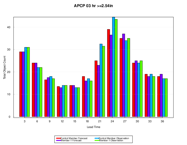
Figure 9.1 Example Bar Plot created by METviewer.
Here is the associated xml for this example. It can be copied into an empty file and saved to the desktop then uploaded into the system by clicking on the “Load XML” button in the upper-right corner of the GUI. This XML can be downloaded from this link: bar_plots_xml.xml.
<?xml version="1.0" encoding="UTF-8" standalone="no"?>
<plot_spec>
<connection>
<host>mohawk</host>
<database>mv_hrrr_sppmp_test</database>
<user>******</user>
<password>******</password>
<management_system>mariadb</management_system>
</connection>
<rscript>/usr/local/R/bin/Rscript</rscript>
<folders>
<r_tmpl>/opt/vxwww/tomcat/webapps/metviewer//R_tmpl</r_tmpl>
<r_work>/opt/vxwww/tomcat/webapps/metviewer//R_work</r_work>
<plots>/d2/www/dtcenter/met/metviewer_output//plots</plots>
<data>/d2/www/dtcenter/met/metviewer_output//data</data>
<scripts>/d2/www/dtcenter/met/metviewer_output//scripts</scripts>
</folders>
<plot>
<template>bar_plot.R_tmpl</template>
<dep>
<dep1>
<fcst_var name="APCP_03">
<stat>CNT_FAA</stat>
<stat>CNT_OAA</stat>
</fcst_var>
</dep1>
<dep2/>
</dep>
<series1>
<field name="model">
<val>HRRR_sppmp_mem0_hrconus</val>
<val>HRRR_sppmp_mem1_hrconus</val>
</field>
</series1>
<series2/>
<plot_fix>
<field equalize="false" name="fcst_thr">
<set name="fcst_thr_0">
<val>>=2.54</val>
</set>
</field>
</plot_fix>
<plot_cond/>
<indep equalize="false" name="fcst_lead">
<val label="3" plot_val="">30000</val>
<val label="6" plot_val="">60000</val>
<val label="9" plot_val="">90000</val>
<val label="12" plot_val="">120000</val>
<val label="15" plot_val="">150000</val>
<val label="18" plot_val="">180000</val>
<val label="21" plot_val="">210000</val>
<val label="24" plot_val="">240000</val>
<val label="27" plot_val="">270000</val>
<val label="30" plot_val="">300000</val>
<val label="33" plot_val="">330000</val>
<val label="36" plot_val="">360000</val>
</indep>
<plot_stat>median</plot_stat>
<tmpl>
<data_file>plot_20200918_194945.data</data_file>
<plot_file>plot_20200918_194945.png</plot_file>
<r_file>plot_20200918_194945.R</r_file>
<title>APCP 03 hr >=2.54in</title>
<x_label>Lead Time</x_label>
<y1_label>Total Object Count</y1_label>
<y2_label/>
<caption/>
<job_title/>
<keep_revisions>false</keep_revisions>
<listdiffseries1>list()</listdiffseries1>
<listdiffseries2>list()</listdiffseries2>
</tmpl>
<execution_type>Rscript</execution_type>
<event_equal>false</event_equal>
<vert_plot>false</vert_plot>
<x_reverse>false</x_reverse>
<num_stats>false</num_stats>
<indy1_stag>false</indy1_stag>
<indy2_stag>false</indy2_stag>
<grid_on>true</grid_on>
<sync_axes>false</sync_axes>
<dump_points1>false</dump_points1>
<dump_points2>false</dump_points2>
<log_y1>false</log_y1>
<log_y2>false</log_y2>
<varianceinflationfactor>false</varianceinflationfactor>
<plot_type>png16m</plot_type>
<plot_height>8.5</plot_height>
<plot_width>11</plot_width>
<plot_res>72</plot_res>
<plot_units>in</plot_units>
<mar>c(8,4,5,4)</mar>
<mgp>c(1,1,0)</mgp>
<cex>1</cex>
<title_weight>2</title_weight>
<title_size>1.4</title_size>
<title_offset>-2</title_offset>
<title_align>0.5</title_align>
<xtlab_orient>1</xtlab_orient>
<xtlab_perp>-0.75</xtlab_perp>
<xtlab_horiz>0.5</xtlab_horiz>
<xtlab_freq>0</xtlab_freq>
<xtlab_size>1</xtlab_size>
<xlab_weight>1</xlab_weight>
<xlab_size>1</xlab_size>
<xlab_offset>2</xlab_offset>
<xlab_align>0.5</xlab_align>
<ytlab_orient>1</ytlab_orient>
<ytlab_perp>0.5</ytlab_perp>
<ytlab_horiz>0.5</ytlab_horiz>
<ytlab_size>1</ytlab_size>
<ylab_weight>1</ylab_weight>
<ylab_size>1</ylab_size>
<ylab_offset>-2</ylab_offset>
<ylab_align>0.5</ylab_align>
<grid_lty>3</grid_lty>
<grid_col>#cccccc</grid_col>
<grid_lwd>1</grid_lwd>
<grid_x>listX</grid_x>
<x2tlab_orient>1</x2tlab_orient>
<x2tlab_perp>1</x2tlab_perp>
<x2tlab_horiz>0.5</x2tlab_horiz>
<x2tlab_size>0.8</x2tlab_size>
<x2lab_size>0.8</x2lab_size>
<x2lab_offset>-0.5</x2lab_offset>
<x2lab_align>0.5</x2lab_align>
<y2tlab_orient>1</y2tlab_orient>
<y2tlab_perp>0.5</y2tlab_perp>
<y2tlab_horiz>0.5</y2tlab_horiz>
<y2tlab_size>1</y2tlab_size>
<y2lab_size>1</y2lab_size>
<y2lab_offset>1</y2lab_offset>
<y2lab_align>0.5</y2lab_align>
<legend_box>o</legend_box>
<legend_inset>c(0, -.25)</legend_inset>
<legend_ncol>2</legend_ncol>
<legend_size>0.8</legend_size>
<caption_weight>1</caption_weight>
<caption_col>#333333</caption_col>
<caption_size>0.8</caption_size>
<caption_offset>3</caption_offset>
<caption_align>0</caption_align>
<ci_alpha>0.05</ci_alpha>
<plot_ci>c("none","none","none","none")</plot_ci>
<show_signif>c(FALSE,FALSE,FALSE,FALSE)</show_signif>
<plot_disp>c(TRUE,TRUE,TRUE,TRUE)</plot_disp>
<colors>c("#ff0000FF","#8000ffFF","#00aaffFF","#55ff00FF")</colors>
<pch>c(20,20,20,20)</pch>
<type>c("b","b","b","b")</type>
<lty>c(1,1,1,1)</lty>
<lwd>c(1,1,1,1)</lwd>
<con_series>c(1,1,1,1)</con_series>
<order_series>c(1,2,3,4)</order_series>
<plot_cmd/>
<legend>c("Control Member Forecast","Member 1 Forecast","Control Member Observation","Member 1 Observation")</legend>
<y1_lim>c()</y1_lim>
<x1_lim>c()</x1_lim>
<y1_bufr>0.04</y1_bufr>
<y2_lim>c()</y2_lim>
<box_pts>false</box_pts>
<box_outline>false</box_outline>
<box_notch>false</box_notch>
<box_avg>false</box_avg>
<box_boxwex/>
</plot>
</plot_spec>